Note
Click here to download the full example code
Matrix Multiplication
In this tutorial, you will write a 25-lines high-performance FP16 matrix multiplication kernel that achieves performance on par with cuBLAS. You will specifically learn about:
Block-level matrix multiplications
Multi-dimensional pointer arithmetic
Program re-ordering for improved L2 cache hit rate
Automatic performance tuning
Motivations
Matrix multiplications are a key building block of most modern high-performance computing systems. They are notoriously hard to optimize, hence their implementation is generally done by hardware vendors themselves as part of so-called “kernel libraries” (e.g., cuBLAS). Unfortunately, these libraries are often proprietary and cannot be easily customized to accomodate the needs of modern deep learning workloads (e.g., fused activation functions). In this tutorial, you will learn how to implement efficient matrix multiplications by yourself with Triton, in a way that is easy to customize and extend.
Roughly speaking, the kernel that we will write will implement the following blocked algorithm:
# do in parallel
for m in range(0, M, BLOCK_M):
  # do in parallel
  for n in range(0, N, BLOCK_N):
    acc = zeros((BLOCK_M, BLOCK_N), dtype=float32)
    for k in range(0, K, BLOCK_K):
      a = A[m : m+BLOCK_M, k : k+BLOCK_K]
      b = B[k : k+BLOCK_K, n : n+BLOCK_N]
      acc += dot(a, b)
    C[m : m+BLOCK_M, n : n+BLOCK_N] = acc;
where each iteration of the doubly-nested for-loop corresponds to a Triton program instance.
Compute Kernel
The above algorithm is, actually, fairly straightforward to implement in Triton.
The main difficulty comes from the computation of the memory locations at which blocks of A and B must be read in the inner loop. For that, we need multi-dimensional pointer arithmetics.
Pointer Arithmetics
For a row-major 2D tensor X, the memory location of X[i, j] is given by &X[i, j] = X + i*stride_x_0 + j*stride_x_1.
Therefore, blocks of pointers for A[m : m+BLOCK_M, k:k+BLOCK_K] and B[k : k+BLOCK_K, n : n+BLOCK_N] can be defined in pseudo-code as:
&A[m : m+BLOCK_M, k:k+BLOCK_K] =  A + (m : m+BLOCK_M)[:, None]*A.stride(0) + (k : k+BLOCK_K)[None, :]*A.stride(1);
&B[k : k+BLOCK_K, n:n+BLOCK_N] =  B + (k : k+BLOCK_K)[:, None]*B.stride(0) + (n : n+BLOCK_N)[None, :]*B.stride(1);
Which means that pointers for blocks of A and B can be initialized (i.e., k=0) in Triton as:
pid_m = triton.program_id(0)
pid_n = triton.program_id(1)
rm = pid_m * BLOCK_M + triton.arange(0, BLOCK_M)
rn = pid_n * BLOCK_N + triton.arange(0, BLOCK_N)
rk = triton.arange(0, BLOCK_K)
// pointer for A operand
pa = A + (rm[:, None] * stride_a_0 + rk[None, :] * stride_a_1);
// pointer for B operand
pb = B + (rk[:, None] * stride_b_0 + rn[None, :] * stride_b_1);
And then updated in the inner loop as follows:
pa += BLOCK_K * stride_a_1;
pb += BLOCK_K * stride_b_0;
L2 Cache Optimizations
As mentioned above, each program instance computes an [BLOCK_M, BLOCK_N] block of C.
It is important to remember that the order in which these blocks are computed does matter, since it affects the L2 cache hit rate of our program.
And unfortunately, a simple row-major ordering
pid = triton.program_id(0);
grid_m = (M + BLOCK_M - 1) // BLOCK_M;
grid_n = (N + BLOCK_N - 1) // BLOCK_N;
pid_m = pid / grid_n;
pid_n = pid % grid_n;
is just not going to cut it.
One possible solution is to launch blocks in an order that promotes data reuse.
This can be done by ‘super-grouping’ blocks in groups of GROUP_M rows before switching to the next column:
pid = triton.program_id(0);
width = GROUP_M * grid_n;
group_id = pid // width;
# we need to handle the case where M % (GROUP_M*BLOCK_M) != 0
group_size = min(grid_m - group_id * GROUP_M, GROUP_M);
pid_m = group_id * GROUP_M + (pid % group_size);
pid_n = (pid % width) // (group_size);
In practice, this can improve the performance of our matrix multiplication kernel by >10% on some hardware architecture (e.g., 220 to 245 TFLOPS on A100).
Final Result
import torch
import triton
import triton.language as tl

# %
# :code:`triton.jit`'ed functions can be auto-tuned by using the `triton.autotune` decorator, which consumes:
#   - A list of :code:`triton.Config` objects that define different configurations of meta-parameters (e.g., BLOCK_M) and compilation options (e.g., num_warps) to try
#   - A autotuning *key* whose change in values will trigger evaluation of all the provided configs

@triton.autotune(
    configs=[
        triton.Config({'BLOCK_M': 128, 'BLOCK_N': 256, 'BLOCK_K': 32, 'GROUP_M': 8}, num_stages=3, num_warps=8),
        triton.Config({'BLOCK_M': 256, 'BLOCK_N': 128, 'BLOCK_K': 32, 'GROUP_M': 8}, num_stages=3, num_warps=8),
        triton.Config({'BLOCK_M': 256, 'BLOCK_N': 64,  'BLOCK_K': 32, 'GROUP_M': 8}, num_stages=4, num_warps=4),
        triton.Config({'BLOCK_M': 64 , 'BLOCK_N': 256, 'BLOCK_K': 32, 'GROUP_M': 8}, num_stages=4, num_warps=4),\
        triton.Config({'BLOCK_M': 128, 'BLOCK_N': 128, 'BLOCK_K': 32, 'GROUP_M': 8}, num_stages=4, num_warps=4),\
        triton.Config({'BLOCK_M': 128, 'BLOCK_N': 64 , 'BLOCK_K': 32, 'GROUP_M': 8}, num_stages=4, num_warps=4),\
        triton.Config({'BLOCK_M': 64 , 'BLOCK_N': 128, 'BLOCK_K': 32, 'GROUP_M': 8}, num_stages=4, num_warps=4),
        triton.Config({'BLOCK_M': 128, 'BLOCK_N': 32 , 'BLOCK_K': 32, 'GROUP_M': 8}, num_stages=4, num_warps=4),\
        triton.Config({'BLOCK_M': 64 , 'BLOCK_N': 32 , 'BLOCK_K': 32, 'GROUP_M': 8}, num_stages=5, num_warps=2),\
        triton.Config({'BLOCK_M': 32 , 'BLOCK_N': 64 , 'BLOCK_K': 32, 'GROUP_M': 8}, num_stages=5, num_warps=2),
        #triton.Config({'BLOCK_M': 64, 'BLOCK_N': 128, 'BLOCK_K': 32, 'GROUP_M': 8}, num_warps=4),
    ],
    key=['M', 'N', 'K'],
)
# %
# We can now define our kernel as normal, using all the techniques presented above
@triton.jit
def _matmul(A, B, C, M, N, K, stride_am, stride_ak, stride_bk, stride_bn, stride_cm, stride_cn, **META):
    # extract meta-parameters
    BLOCK_M = META['BLOCK_M']
    BLOCK_N = META['BLOCK_N']
    BLOCK_K = META['BLOCK_K']
    GROUP_M = 8
    # matrix multiplication
    pid = tl.program_id(0)
    grid_m = (M + BLOCK_M - 1) // BLOCK_M
    grid_n = (N + BLOCK_N - 1) // BLOCK_N
    # re-order program ID for better L2 performance
    width = GROUP_M * grid_n
    group_id = pid // width
    group_size = min(grid_m - group_id * GROUP_M, GROUP_M)
    pid_m = group_id * GROUP_M + (pid % group_size)
    pid_n = (pid % width) // (group_size)
    # do matrix multiplication
    rm = pid_m * BLOCK_M + tl.arange(0, BLOCK_M)
    rn = pid_n * BLOCK_N + tl.arange(0, BLOCK_N)
    rk = tl.arange(0, BLOCK_K)
    A = A + (rm[:, None] * stride_am + rk[None, :] * stride_ak)
    B = B + (rk[:, None] * stride_bk + rn[None, :] * stride_bn)
    acc = tl.zeros((BLOCK_M, BLOCK_N), dtype=tl.float32)
    for k in range(K, 0, -BLOCK_K):
        a = tl.load(A)
        b = tl.load(B)
        acc += tl.dot(a, b)
        A += BLOCK_K * stride_ak
        B += BLOCK_K * stride_bk
    # triton can accept arbitrary activation function
    # via metaparameters!
    if META['ACTIVATION']:
        acc = META['ACTIVATION'](acc)
    # rematerialize rm and rn to save registers
    rm = pid_m * BLOCK_M + tl.arange(0, BLOCK_M)
    rn = pid_n * BLOCK_N + tl.arange(0, BLOCK_N)
    C = C + (rm[:, None] * stride_cm + rn[None, :] * stride_cn)
    mask = (rm[:, None] < M) & (rn[None, :] < N)
    tl.store(C, acc, mask=mask)


# we can fuse `leaky_relu` by providing it as an `ACTIVATION` meta-parameter in `_matmul`
@triton.jit
def leaky_relu(x):
    return tl.where(x >= 0, x, 0.01*x)
We can now create a convenience wrapper function that only takes two input tensors and (1) checks any shape constraint; (2) allocates the output; (3) launches the above kernel
def matmul(a, b, activation=None):
    # checks constraints
    assert a.shape[1] == b.shape[0], "incompatible dimensions"
    assert a.is_contiguous(), "matrix A must be contiguous"
    assert b.is_contiguous(), "matrix B must be contiguous"
    M, K = a.shape
    _, N = b.shape
    # allocates output
    c = torch.empty((M, N), device=a.device, dtype=a.dtype)
    # launch kernel
    grid = lambda META: (triton.cdiv(M, META['BLOCK_M']) * triton.cdiv(N, META['BLOCK_N']), )
    pgm = _matmul[grid](
        a, b, c, M, N, K, \
        a.stride(0), a.stride(1), b.stride(0), b.stride(1), c.stride(0), c.stride(1),\
        ACTIVATION = activation
    )
    # done; return the output tensor
    return c
Unit Test
We can test our custom matrix multiplication operation against a native torch implementation (i.e., cuBLAS)
torch.manual_seed(0)
a = torch.randn((512, 512), device='cuda', dtype=torch.float16)
b = torch.randn((512, 512), device='cuda', dtype=torch.float16)
c_0 = matmul(a, b, activation=None)
c_1 = torch.matmul(a, b)
print(c_0)
print(c_1)
print(triton.testing.allclose(c_0, c_1))
Out:
tensor([[  1.1045, -36.9688,  31.4688,  ..., -11.3984,  24.4531, -32.3438],
        [  6.3555, -19.6094,  34.0938,  ...,  -5.8945,   5.2891,   6.8867],
        [-32.0625,   5.9492,  15.3984,  ..., -21.3906, -23.9844, -10.1328],
        ...,
        [ -5.7031,   7.4492,   8.2656,  ..., -10.6953, -40.0000,  17.7500],
        [ 25.5000,  24.3281,  -8.4688,  ..., -18.9375,  32.5312, -29.9219],
        [ -5.3477,   4.9844,  11.8906,  ...,   5.5898,   6.4023, -17.3125]],
       device='cuda:0', dtype=torch.float16)
tensor([[  1.1045, -36.9688,  31.4688,  ..., -11.3906,  24.4531, -32.3438],
        [  6.3516, -19.6094,  34.0938,  ...,  -5.8906,   5.2812,   6.8828],
        [-32.0625,   5.9531,  15.3984,  ..., -21.4062, -23.9844, -10.1328],
        ...,
        [ -5.7070,   7.4492,   8.2656,  ..., -10.6953, -40.0000,  17.7500],
        [ 25.5000,  24.3438,  -8.4609,  ..., -18.9375,  32.5312, -29.9219],
        [ -5.3477,   4.9805,  11.8828,  ...,   5.5859,   6.4023, -17.3125]],
       device='cuda:0', dtype=torch.float16)
tensor(True, device='cuda:0')
Benchmark
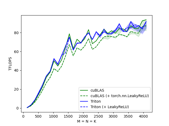
Square Matrix Performance
We can now compare the performance of our kernel against that of cuBLAS. Here we focus on square matrices, but feel free to arrange this script as you wish to benchmark any other matrix shape.
@triton.testing.perf_report(
    triton.testing.Benchmark(
        x_names=['M', 'N', 'K'],  # argument names to use as an x-axis for the plot
        x_vals=[128 * i for i in range(1, 33)],  # different possible values for `x_name`
        line_arg='provider',  # argument name whose value corresponds to a different line in the plot
        line_vals=['cublas', 'cublas + relu', 'triton', 'triton + relu'],  # possible values for `line_arg``
        line_names=["cuBLAS", "cuBLAS (+ torch.nn.LeakyReLU)", "Triton", "Triton (+ LeakyReLU)"],  # label name for the lines
        styles=[('green', '-'), ('green', '--'), ('blue', '-'), ('blue', '--')],  # line styles
        ylabel="TFLOPS",  # label name for the y-axis
        plot_name="matmul-performance",  # name for the plot. Used also as a file name for saving the plot.
        args={}
    )
)
def benchmark(M, N, K, provider):
    a = torch.randn((M, K), device='cuda', dtype=torch.float16)
    b = torch.randn((K, N), device='cuda', dtype=torch.float16)
    if provider == 'cublas':
        ms, min_ms, max_ms = triton.testing.do_bench(lambda: torch.matmul(a, b))
    if provider == 'triton':
        ms, min_ms, max_ms = triton.testing.do_bench(lambda: matmul(a, b))
    if provider == 'cublas + relu':
        torch_relu = torch.nn.ReLU(inplace=True)
        ms, min_ms, max_ms = triton.testing.do_bench(lambda: torch_relu(torch.matmul(a, b)))
    if provider == 'triton + relu':
        ms, min_ms, max_ms = triton.testing.do_bench(lambda: matmul(a, b, activation=leaky_relu))
    perf = lambda ms: 2 * M * N * K * 1e-12 / (ms * 1e-3)
    return perf(ms), perf(max_ms), perf(min_ms)


benchmark.run(show_plots=True, print_data=True)
Out:
matmul-performance:
         M     cuBLAS  ...     Triton  Triton (+ LeakyReLU)
0    128.0   0.455111  ...   0.512000              0.512000
1    256.0   2.730667  ...   3.276800              3.276800
2    384.0   7.372800  ...   8.507077              8.507077
3    512.0  14.563555  ...  16.384000             15.420235
4    640.0  22.260869  ...  24.380953             24.380953
5    768.0  32.768000  ...  34.028308             34.028308
6    896.0  37.971025  ...  39.025776             39.025776
7   1024.0  49.932191  ...  52.428801             52.428801
8   1152.0  44.566925  ...  46.656000             45.938215
9   1280.0  51.200001  ...  56.109587             56.109587
10  1408.0  64.138541  ...  65.684049             58.601554
11  1536.0  78.643199  ...  75.296679             75.296679
12  1664.0  62.929456  ...  61.636381             61.636381
13  1792.0  72.983276  ...  68.953520             68.533074
14  1920.0  69.120002  ...  69.120002             69.467336
15  2048.0  73.584279  ...  75.573044             75.234154
16  2176.0  83.155572  ...  79.855747             79.855747
17  2304.0  68.251065  ...  72.607513             72.828879
18  2432.0  71.305746  ...  80.963875             80.963875
19  2560.0  77.649287  ...  76.740048             75.155963
20  2688.0  83.552988  ...  81.053536             83.552988
21  2816.0  79.154642  ...  78.726003             78.161663
22  2944.0  81.967162  ...  78.605729             79.737653
23  3072.0  79.415291  ...  81.825298             83.391907
24  3200.0  84.210524  ...  89.385477             85.333333
25  3328.0  83.905938  ...  81.346098             81.808290
26  3456.0  81.108217  ...  81.026701             85.133652
27  3584.0  87.381330  ...  91.750399             85.064084
28  3712.0  84.159518  ...  85.309435             88.326564
29  3840.0  84.550462  ...  87.217666             87.493673
30  3968.0  92.442373  ...  84.680037             83.692683
31  4096.0  93.662059  ...  91.867031             91.616198

[32 rows x 5 columns]
Total running time of the script: ( 2 minutes 12.186 seconds)